The goal of most sequencing experiments is to identify differences in gene expression between biological conditions such as the influence of a disease-linked genetic mutation or drug treatment. Fitting the correct statistical model to the data is an essential step before making inferences about differentially expressed genes. The negative binomial (NB) distribution has emerged as the model of choice to fit sequencing data. While the NB distribution is bread-and-butter to a statistician, the average experimental biologist may not be very familiar with it.
A first intuition
In a standard sequencing experiment (RNA-Seq), we map the sequencing reads to the reference genome and count how many reads fall within a given gene (or exon). This means that the input for the statistical analysis are discrete non-negative integers (“counts”) for each gene in each sample. The total number of reads for each sample tends to be in the millions, while the counts per gene vary considerably but tend to be in the tens, hundreds or thousands. Therefore, the chance of a given read to be mapped to any specific gene is rather small. Discrete events that are sampled out of a large pool with low probability sounds very much like a Poisson process. And indeed it is. In fact, earlier iterations of RNA-Seq analysis modeled sequencing data as a Poisson distribution. There is one problem, however. The variability of read counts in sequencing experiments tends to be larger than the Poisson distribution allows.
A fundamental property of the Poisson distribution is that its variance is equal to the mean. Here I plotted the gene-wise means versus their variance of the “bottomly” experiment provided by the ReCount project. The code to produce this plot can be found on Github.
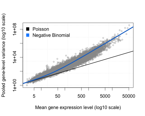
It is obvious that the variance of counts is generally greater than their mean, especially for genes expressed at a higher level. This phenomenon is called “overdispersion“. The NB distribution is similar to a Poisson distribution but has an extra parameter called the “clumping” or “dispersion” parameter. It is like a Poisson distribution with more variance. Note, how the NB estimates of the mean-variance relationship (blue line) fits the observed values quite well. Thus, a reasonable first intuition of why the NB distribution is a proper way of fitting count data is that the dispersion parameter allows the extra wiggle room to model the “extra” variance that we empirically observe in RNA-Seq experiments.
A more rigorous justification
There are two mathematically equivalent formulations of the NB distribution. In its traditional form, which I will mention only for the sake of completion, the NB distribution estimates the probability of having a number of failures until a specified number of successes occur. An example for an application would be the expected number of games a striker goes without a goal (“failure”) before scoring (“success”). Note that, “success” and “failure” are not value judgements but just the two outcomes of a Bernoulli process and therefore interchangeable. Whenever you see the NB distribution used in this form, pay close attention to what is defined as a “success” and a “failure”. In is a common point of notational confusion. This definition is not terribly useful for understanding how the NB distribution relates to RNA-Seq count data.
The second definition sounds more intimidating but is much more useful. The NB distribution can be defined as a Poisson-Gamma mixture distribution. This means that the NB distribution is a weighted mixture of Poisson distributions where the rate parameter 
While it is convenient to have a distribution that fits our empirical observations it is not quite satisfying without a more theoretical justification. When comparing samples of different conditions we usually have multiple replicates of each condition. Those replicates need to be independent for statistical inference to be valid. Such replicates are called “biological” replicates because they come from independent animals, dishes, or cultures. In contrast, splitting a sample in two and running it through the sequencer twice would be a “technical” replicate. In general, there is more variance associated with biological replicates than technical replicates. If we assume that our samples are biological replicates, it is not surprising that the same transcript is present at slightly different levels in each sample, even under the same conditions. In other words, the Poisson process in each sample has a slightly different expected count parameter. This is the source of the “extra” variance (overdispersion) we observe in sequencing data. In the framework of the NB distribution, it is accounted for by allowing Gamma-distributed uncertainty about the expected counts (the Poisson rate) for each gene. Conversely, if we were to deal with technical replicates, there should be no overdispersion and a simple Poisson model would be adequate.
The variance (dispersion) 


From this formula it is evident that the dispersion is always greater than the mean for 

Dispersion estimates
Finally, a short note on the practical implications of estimating the dispersion of sequencing data. In a standard sequencing experiment, we have to be content with few biological replicates per condition due to the high costs associated with sequencing experiments and the large amount of time that goes into library preparations. This makes the gene-wise estimates of dispersion rather unreliable. Modern RNA-Seq analysis tools such as DESeq2 and edgeR combine the gene-wise dispersion estimate with an estimate of the expected dispersion rate based on all genes. This Bayesian “shrinkage” of the variance has already been applied successfully in microarray analysis. Although the implementation of this method varies between analysis tools, the concept of using information from the whole data set has emerged as a powerful technique to mitigate the shortcomings of having few replicates.
